Latex: Indent an entire paragraph

Here is a good post: https://tex.stackexchange.com/questions/35933/indenting-a-whole-paragraph

My way is from this post. This way is the simplest. No additional package is needed.

\setlength{\leftskip}{2em}
Paragraph1

Paragraph2

Remarks:

All the following paragraphs are affected by \setlength{\leftskip}{2em}

If you want to stop the effect, you can set \setlength{\leftskip}{0em}

If this is within an environment such as mdframed, you don’t need to set it back to 0em, because it will do automatically. That is the command would not affect the code our side the environment.

Note that \quad=1em, \qquad=2em!!

Latex ctex中文下划线换行

如果是英文的，参考下面：https://tex.stackexchange.com/questions/9550/why-does-underlined-text-not-get-wrapped-once-it-hits-the-end-of-a-line

其中有一个：使用ulem package 的\uline命令，\usepackage{ulem}

我在中文上面实验发现还是不行，一大段话能分成两行，但是第一行还是很长。

如果是中文的，应该用下面的方法：即中文化的ulem package

\usepackage{CJKulem}

\normalem

\uline{中文 }

注意如果不适用\normalem这个命令，那么emph就会变成下划线。

发现很有意思的一点，那就是中文其实没法斜体，即使用emph或者textit也无效，即使winedt里面显示是斜体，但是编译出来不是，有的人说汉字压根就没有斜体

latex ctex 中文参考文献乱码

别人给我的一个文件，编译出问题，查了一些文献，自己尝试了一下，解决了：

1. 中文参考文献的label还是用英文的例如\cite{zhao2020}而不是\cite{赵2020}，有的软件编译没问题，有的有问题

2. 之前给我的一个bib，编译后参考文献乱码；后来用ctex另存为utf8还是乱码；后来把内容copy到一个txt文件，再把文件扩展名修改为.bib，然后再另存为utf8，编译通过没有乱码了。所以原文件不知道发生了什么，需要另起炉灶。

Ctex MiKTeX latex package自动更新

这是不错的介绍

https://blog.csdn.net/weixin_42268054/article/details/88898984

问题：之前一切正常，最近不正常了，出现了sty无法加载。原因是之前选择自动下载的服务器down掉了。

找到Miktex Console（在win10搜索即可），打开里面settings-》packages are installed from->change->next，然后从列表选择，一般选择更新时间最新的，最上面的

************************************************************************************

之前关于tcolorbox的编译是可以的，现在不行了，特别是breakable的选项

\usepackage{tcolorbox}
%\tcbuselibrary{breakable}

\begin{tcolorbox}[breakable,title=The coefficients in the Robbins-Monro algorithm, beforeupper={\parindent15pt\noindent}]

latex text box

It is sometimes required to plot a bounding box around some text in a latex document. It is very simple.

\usepackage{tcolorbox}[
enhanced,
breakable,
frame hidden,
overlay broken = {
\draw[line width=0.5mm, black, rounded corners]
(frame.north west) rectangle (frame.south east);},
]

\begin{tcolorbox}

\end{tcolorbox}

如果最大限度的压缩PDF特别是里面的图片的大小

第一步：save as-> reduced size PDF

这个可能无法满足要求。

第二步：把PDF中扫描的图片页面单独提取出来成为PDF，再进一步另存为jpg图片，jpg图片已经没有PDF的清楚了，然后在把jpg图片combine并转成PDF，最后再用PDF自带的reduced size PDF功能即可大大压缩。

例子：我一个PDF全部是扫描图片5兆多，转成多个jpg图片后一共成了9兆，再合并成PDF也还是9兆多，但是reduced size PDF后变成了2兆多。最后图片质量会下降。

另外这样最后的PDF和原来PDF的尺寸是样的。如果是另存为PNG（质量比较高），再压缩图片，再转PDF得到的文件和原来文件放到一起页面会很小。

How to sample from a discrete distribution Matlab

function sample=fcn_SampleFromDistribution(variable, PDF)
varNum=max(size(variable)); % number of variables
CDF=cumsum(PDF); % the values increase from 0 to 1
randnum=rand; % a random number uniformly drawn from [0,1]
for i=1:varNum
  if randnum<=CDF(i)
    sample=variable(i);
    break;
  end
end

Example:

variable=[2 3 4 5 6]; % must be monotonic
PDF=[0.1 0.1 0.1 0.1 0.6]; % the sum must be 1

One note: after you get a random number using rand function, you should compare with the values in CDF. You should check from the smallest values. If randnum is smaller than a value, then the sample would correspond to the value at the same position in the variable array. Note that when you compare CDF and randnum, should not choose the closest value, instead choose the closest but larger value in CDF.

Two good articles about the problem:

• https://sciencehouse.wordpress.com/2015/06/20/sampling-from-a-probability-distribution/
• https://www.mathworks.com/matlabcentral/fileexchange/21912-sampling-from-a-discrete-distribution

 

Latex/Beamer支持中文slide

为了支持中文，在我原来代码基础之上需要做下面几件事：

1. 把下面的代码添加到\begin{document}之前

其中开头几行是支持中文字体，后面是把章节目录等英文的换成中文的。

%=========support Chinese
\usepackage{CJK}
%gbsn简体宋 gkai简体楷 bsmi繁体宋 bkai繁体楷
\usepackage{CJKnumb}
%\titleformat{\chapter}[hang]{\LARGE\bfseries}{\chaptername}{1em}{}
%\renewcommand{\chaptername}{第\CJKnumber{\thechapter}章}
%\titleformat{\section}[hang]{\LARGE\bfseries}{\sectionname}{1em}{}
%\renewcommand{\sectionname}{第\CJKnumber{\thesection}章}
%\renewcommand{\contentsname}{目\quad 录}
%\renewcommand\contentsname{目录}
%\renewcommand{\abstractname}{摘\quad 要}
%\renewcommand\listfigurename{图片索引}
%\renewcommand\listtablename{表格索引}
%\newcommand{\loflabel}{图}
%\newcommand{\lotlabel}{表}
%\renewcommand{\figurename}{图}
%\renewcommand{\tablename}{表}
%\renewcommand{\refname}{参考文献}
%\renewcommand{\bibname}{参考文献}
%=========support Chinese

2. 在正文部分加上下面代码：支持的字体有gbsn简体宋 gkai简体楷 bsmi繁体宋 bkai繁体楷等多种

\begin{document}

\begin{CJK*}{UTF8}{gbsn} % \end{CJK*} is at the end
\hypersetup{CJKbookmarks=true}

\begin{frame}
\frametitle{研究兴趣}
测试
\end{frame}

\end{CJK*}

3. 把正文main.tex另存为UTF-8格式，把其它含有汉字的tex文件例如title_page.tex也另存为UTF-8，否则直接报错就是invalid character

如果是一个有汉字的，你想去除掉汉字并且回归原来的纯英文编译和格式，只需要把里面的汉字全部删除，下次打开不需要专门与utf-8格式打开了，不需要专门另存为普通模式。

4. 编译器直接按F9即可，即PDFTexify即可，其它的例如XeLatex反而不行（没有错误，但是编译完没有弹出PDF）

注意这里是针对Beamer，如果是中文论文，那么编译器必须要用XeLatex

Matlab支持中文路径名称

有时候文件夹的名称是中文的（文件的名称不是中文的），Matlab可能不支持。

修改win10的region里面的format为中文，重新启动matlab就行了

注意是format设置为中文不只是country

Latex Missing $ inserted

2022-03-29

A similar bug appeared today. A very simple paragraph leads to an error. I am sure there is no mistake. The error disappeared when I comment the paragraph. However, later in a while, the error emerges again even if the paragraph is still commented.

Finally the problem is solved when I follow the error hint generated by the system. That is I embed “itemize” inside another itemize. Actually this should work. But today it just does not work. After I removed the outer itemize environment, the error disappeared forever.

***************************************************************

This error bugged me for a long time.

What’s really wired is that if you add one sentence then the error pops out, if you remove that sentence, the error disappears. But that sentence is a plain text sentence! This is really wired. In fact, if you add another sentence, you may also see the error. It is random, and that’s why it is really a headache!

The conclusion is that I finally solved it. The problem causing the error is that I used some symbols like underscores “_” in some variables!

\chapter[chapter_bearingRigidity]{Bearing Rigidity Theory}

is problematic! Sometimes it works, and sometimes it does not!

\chapter[chapterBearingRigidity]{Bearing Rigidity Theory}

is good!

We know that in many programing languages such as Matlab or C, we can use underscores in variables without any problems.

The fundamental reason in Latex is that Latex may think _ as a math symbol: subscript!! That’s why it asks you to insert $

I was inspired by this post:

https://stackoverflow.com/questions/2476831/getting-the-error-missing-inserted-in-latex

Win10 switch input shortcut

I have one Chinese input and one English input. The standard and default way to change between them is shift+alt, while I always use shift+ctrl (this is the default shortcut of windows before).

So how to change the shortcut?

The ultimate position to change it is in the “Text services and input languages” dialog window.

1. How to find this dialog window? There are different ways. For example, in some windows systems, you can find the Language option, then you can find it. But in my case, it is very strange and it is located at

Devices->Typing->Advanced keyboard settings->Language bar options

2. If you see this dialog window, how to set?

Advanced keyboard settings tab->Between input languages->Change Key Sequence

 

Useful Tricks in Microsoft Word

Return to the location you edited last time

This is especially useful if you are editing a long document.

• Method 1: Shift+F5, this is the simplest way
• Method 2: On the right hand side of MS word 2018, there will be a flag for this purpose.

Change list level: very useful!!

alt+shift+leftarrow or rightarrow

 

 

Latex color text

If you would like to change the color of some text in latex, there are two ways:

• \textcolor{<color>}{...}

Example:

\definecolor{myColor}{RGB}{0,0,200}
\newcommand{\blue}{\textcolor{blue}}

\blue{xxxx}

This way it is very simple to change the color of some text. However, its problem is that it does not allow line breaks. It would be very annoying to use this command if you would like to change the color of many paragraphs.

• {\color{<color>}...}

Example:

\usepackage{xcolor}

{\color{blue}

Paragraph 1 xxx
paragraph 2 xxx
}

This way is powerful because you can change the color an entire section if needed. Note that here you do not need to define the color blue, it is a default color.

Latex: multiple columns with different/uneven width

Some methods that do NOT work:

First,

\usepackage{multicol}
\begin{multicols}{2}
\end{multicols}

The problem of this method is that you cannot adjust the column width, which is automatically calculated by the package.

Second,

\usepackage{vwcol}
\begin{vwcol}[widths={0.6,0.4}]
\end{vwcol}

The problem is that it simply does not work properly and I didn’t spend too much time digging out. The supporting websites are not many.

Third,

using tables. The problem is that when I insert sections or other environments in tables, there were errors. I guess table is after all a local environment. It is not suitable to put all the document in tables.

Method that works:

minipage:

\noindent
\begin{minipage}[c]{0.6\linewidth}
xxx
\end{minipage} % no space if you would like to put them side by side
\begin{minipage}[c]{0.3\linewidth}
xxx
\end{minipage}

Latex支持中文和修改中文字体

如何设置CTex使之支持中文：

很好的文章:

http://gaolei786.github.io/latex/helloctex.html

https://wenku.baidu.com/view/dbd74b5b1611cc7931b765ce05087632311274b2.html

上面两个链接是一个文章。

要点是：

1. 保存类型：类型选”UTF-8”，后缀选择***.tex。也许在下面的{ctex}前面加上[UTF8]也可以。
2. \usepackage[UTF8]{ctex} %加载包，因为我们在用中文写文档
3. 就可以直接在WinEdit中对它编译。首先要选择合适的编译器：XeLatex, 这个编译器对中文支持比较好

我已经成功实现中文输入。不过每次需要点击XeLatex编译，而且不会自动弹出来PDF，需要手动点击PDF预览按钮。

修改F9快捷键：F9默认的是pdflatex来编译，如果我们希望使用xelatex来编译可以修改F9快捷键。注意：一般性的修改快捷键的方式比较复杂，我们直线想修改编辑器，可以通过下面方式修改。Option (menu)->Exaction Modes->Tex Options (tab)->Default PDFTexify Engine:

• 默认值是pdflatex.exe
• 改成xelatex.exe即可

我的WinEdt的版本是7，还需要每次指定F9触发的编译器. 更高级的版本可以支持更方便的修改，即只是触发下拉列表里面选择的编译器。https://tex.stackexchange.com/questions/169493/change-default-compiler-by-drop-down-button-in-winedt

把图的Figure变成汉字“图”：\renewcommand{\figurename}{图}

解决“error reading”无法打开的问题：如果是中文的，并且是UTF-8格式的tex，直接双击文件无法打开，会报错。这时候先打开winedt软件，然后open菜单，在选择文件的窗口右下角选择“UTF-8”格式，而非默认的*.*格式。

修改WinEdt显示的字体：修改font文件里面的

FONT_NAME=”Calibri” //”Calibri” //”Times New Roman”// “SimSun” //default “Courier New”

如何修改中文字体：

下面是我测试完的管用的：

http://blog.csdn.net/programchangesworld/article/details/51429138

要点：

1. 改变字体分为两种，一种是全局改变，一种是局部改变。

\usepackage{CJK}
% 用于全局修改字体
\setCJKmainfont{STXingkai}
% 用于局部修改字体
\setCJKfamilyfont{hwxk}{STXingkai}
\newcommand{\huawenxingkai}{\CJKfamily{hwxk}}

局部修改的方法：{\huawenxingkai 测试字体}

2. 哪些字体可选择：上面是STXingkai是行楷，还有

STCaiyun,华文彩云:style=Regular
YouYuan,幼圆:style=Regular
STHupo,华文琥珀:style=Regular
KaiTi_GB2312,楷体_GB2312:style=Regular
NSimSun,新宋体:style=Regular
FangSong_GB2312,仿宋_GB2312:style=Regular
SimSun,宋体:style=Regular
STXinwei,华文新魏:style=Regular
SimHei,黑体:style=Regular
STXingkai,华文行楷:style=Regular
LiSu,隶书:style=Regular

我上面测试成功的包括：FangSong, SimSun, NSimSun, STXinwei, SimHei

关于字体代码，参见http://kuing.is-programmer.com/posts/32555.html

Latex: usage of subfloat minipage

\begin{figure*}
 \centering
\subfloat[]{
\begin{minipage}[b][][t]{.3\textwidth} % [b] bottom [t] top
\centering
\includegraphics[width=\linewidth]{fig_sim_singleIntegrator_noIntegralStationary_traj}
\includegraphics[width=\linewidth]{fig_sim_singleIntegrator_noIntegralStationary_bearingerror}
\end{minipage}}%
\subfloat[]{
\begin{minipage}[b][][t]{.3\textwidth} % [b] bottom [t] top
\centering
\includegraphics[width=\linewidth]{fig_sim_singleIntegrator_noIntegralMoving_traj}
\includegraphics[width=\linewidth]{fig_sim_singleIntegrator_noIntegralMoving_bearingerror}
\end{minipage}}%
\subfloat[]{
\begin{minipage}[b][][t]{.3\textwidth} % [b] bottom [t] top
\centering
\includegraphics[width=\linewidth]{fig_sim_singleIntegrator_PIMoving_traj}
\includegraphics[width=\linewidth]{fig_sim_singleIntegrator_PIMoving_bearingerror}
\end{minipage}}%
 \caption{The bearing error is $\sum_{(i,j)\in\E}\|g_{ij}-g_{ij}^*\|$.}
 \label{fig_sim_PI_noIntegral}
\end{figure*}

Feedback linearization of Unicycle Model

Keywords: unicycle, single integrator, double integrator, feedback linearization

There are two types of feedback linearization of unicycle models. The first is to obtain a single-integrator model. The second is to obtain a double-integrator model (reference for the double integrator model: Automatica “Distributed formation control of nonholonomic mobile robots without global position measurements”).

my memo: unicycle linearization

Get Euler angles from a rotation matrix

Matlab function:

function rho=fcn_EulerFromRotation(R)
% R is the rotation from body to world frame

% assume -pi/2<tht<pi/2

%R31=-sin(tht)
tht=-asin(R(3,1));

%R32=sin(phi)*cos(tht), R33=cos(phi)*cos(tht)
phi=atan2(R(3,2),R(3,3));

%R21=cos(tht)*sin(psi), R11=cos(tht)*cos(psi)
psi=atan2(R(2,1),R(1,1));

rho=[phi,tht,psi]';

matlab generate the same random number everytime

use the following command before the rand function, you will get the same random number everytime you run the m file.

rand(‘seed’, 0);

rand

Set latex font

The command is:

\renewcommand*\rmdefault{ptm} %ppl

if you want to understand the three letter word: ptm or ppl. Read the table III of this document: http://tug.ctan.org/macros/latex/required/psnfss/psnfss2e.pdf

Here is a good introduction:

Click to access schmidt.pdf

Abbrivation

Theorem -> Thm.
Corollary -> Cor.
See https://en.wikipedia.org/wiki/List_of_mathematical_abbreviations

Chapter -> Chap.

see https://en.wikipedia.org/wiki/List_of_legal_abbreviations

 

Insert Youtube video to powerpoint

Keywords: youtube, video, PPT, powerpoint, starting time

• First, go to youtube and find the video. Then click Share->Embed. You will get a code as below:

• Second, paste the code to word and modify it. Specify the starting and ending times as shown below.

• Third, go to PPT and click Insert->Video->Online Video->From a Video Embed Code (not the Youtube one). Copy and paste and nail it.

 

 

Bearing Laplacian: Matlab code

Bearing Laplacian is important in the area of bearing rigidity. Here is the matlab code to generate the bearing Laplacian of a given network. If the rank of the bearing Laplacian is equal to d*n-d-1, then the network is bearing rigid.

keywords: bearing rigidity, bearing Laplacian

clc;clear;close all
% positions of the nodes in the network
p_all=[0 0 0;
   0 1 0;
   -1 0 0;
   0 0 1]';
d=size(p_all,1); % dimension
n=size(p_all,2); % number of nodes
% The symmetric adjacent matrix
neighborMat=zeros(n,n);
neighborMat(1,2)=1;neighborMat(1,4)=1;
neighborMat(2,3)=1;
neighborMat(3,4)=1;
neighborMat=neighborMat+neighborMat';

% Calculate the bearing Laplacian L
L=zeros(d*n,d*n);
for i=1:n
    for j=1:n
        if neighborMat(i,j)~=0 && i~=j
            pi=p_all(:,i);
            pj=p_all(:,j);
            gij=(pj-pi)/norm(pj-pi);
            Pgij=eye(d)-gij*gij';
            L(d*(i-1)+1:d*(i-1)+d,d*(j-1)+1:d*(j-1)+d)=-Pgij;
            L(d*(i-1)+1:d*(i-1)+d,d*(i-1)+1:d*(i-1)+d)...
             =L(d*(i-1)+1:d*(i-1)+d,d*(i-1)+1:d*(i-1)+d)+Pgij;
        end
    end
end

% See if the rank of L is equal to d*n-d-1. If so, the network is bearing rigid
rank(L)-(d*n-d-1)

A special but useful orthogonal projection matrix

 

See details in the memo

matlab annotation

x=[0.25,0.25];
y=[0.45,0.32];
a=annotation(‘textarrow’,x,y,’String’,’x_{2}(t), x_{14}(t)’);
set(a, ‘color’, myRed, ‘interpreter’, ‘tex’, ‘fontSize’, 15)

Matlab: plot multi-agent formation control

very easy to use!! just copy and paste to your m file and it works!!

Note: set up the input arguments

• x_all_time
• num
• neighborMat

function fcn_myPlot(x_all_time)
global A d n
num=n;
neighborMat=A;
%%%%%%%%%%%%%%%%%%%%%%%%%%%%
graycolor=[0.5 0.5 0.5];
markersize=30;
textsize=25;
finalcolor=[0 0 1]*0.8;
%
figure;
hold on; box on; axis equal
% set label and tick
fontsize=20;
set(gca, 'fontSize', fontsize)
set(get(gca, 'xlabel'), 'String', 'x', 'fontSize', fontsize);
set(get(gca, 'ylabel'), 'String', 'y', 'fontSize', fontsize);
% hide label and tick
% set(gca, 'xtick', [])
% set(gca, 'ytick', [])
% boxcolor=0.7*ones(1,3);
% set(gca, 'xcolor', boxcolor)
% set(gca, 'ycolor', boxcolor)
%%%%%%%%%%%%%%%%%%%%%%%%%%%%%%%%%%%%%%%%%%%%%%%%%%%%%%%%%%%%%%%%
% plot agent trajectory
for i=1:num
    xi_all=x_all_time.signals.values(:,2*i-1);
    yi_all=x_all_time.signals.values(:,2*i);
    plot(xi_all, yi_all, '--', 'color', graycolor);
end
%%%%%%%%%%%%%%%%%%%%%%%%%%%%%%%%%%%%%%%%%%%%%%%%%%%%%%%%%%%%%%%%%%
% initial formation
% for i=1:num
%     for j=i+1:num
%         if neighborMat(i,j)==1
%             pi=x_all_time.signals.values(1,2*i-1:2*i)';
%             pj=x_all_time.signals.values(1,2*j-1:2*j)';
%             line([pi(1),pj(1)], [pi(2),pj(2)], 'linewidth', 2, 'color', graycolor);
%         end
%     end
% end
for i=1:num
    xi_init=x_all_time.signals.values(1,2*i-1);
    yi_init=x_all_time.signals.values(1,2*i);
    plot(xi_init, yi_init, 'o', 'MarkerEdgeColor', graycolor, 'MarkerFaceColor', graycolor, 'markersize', 10)
end
% plot circles and text: initial
for i=1:num
    xi_init=x_all_time.signals.values(1,2*i-1);
    yi_init=x_all_time.signals.values(1,2*i);
    plot(xi_init, yi_init, 'o', ...
        'MarkerSize', markersize,...
        'linewidth', 2,...
        'MarkerEdgeColor', graycolor,...
        'markerFaceColor', 'white');
    text(xi_init, yi_init, num2str(i),...
        'color', graycolor, 'FontSize', textsize, 'horizontalAlignment', 'center', 'FontName', 'times');
end
%%%%%%%%%%%%%%%%%%%%%%%%%%%%%%%%%%%%%%%%%%%%%%%%%%%%%%%%%%%%%%%%%%%%%%%%%%%%%
% final formation
for i=1:num
    for j=i+1:num
        if neighborMat(i,j)==1
            pi=x_all_time.signals.values(end,2*i-1:2*i)';
            pj=x_all_time.signals.values(end,2*j-1:2*j)';
            line([pi(1),pj(1)], [pi(2),pj(2)], 'linewidth', 2, 'color', finalcolor);
        end
    end
end
% plot circles and text: final
for i=1:num
    xi_init=x_all_time.signals.values(end,2*i-1);
    yi_init=x_all_time.signals.values(end,2*i);
    plot(xi_init, yi_init, 'o', ...
        'MarkerSize', markersize,...
        'linewidth', 2,...
        'MarkerEdgeColor', finalcolor,...
        'markerFaceColor', [1 1 1]);
    text(xi_init, yi_init, num2str(i),...
        'color', finalcolor, 'FontSize', textsize, 'horizontalAlignment', 'center', 'FontName', 'times');
end
% % intermediate formation
% for k=1:size(x_all_time.time,1)
%     for i=1:num
%         for j=i+1:num
%             if neighborMat(i,j)==1
%                 pi=x_all_time.signals.values(k,2*i-1:2*i)';
%                 pj=x_all_time.signals.values(k,2*j-1:2*j)';
%                 line([pi(1),pj(1)], [pi(2),pj(2)], 'linewidth', 1, 'color', rand(1,3));
%             end
%         end
%     end
% end
%%%%%%%%%%%%%%%%%%%%%%%%%%%%%%%%%%%%%%%%%%%%%%%%%%%%%%%%%%%%%%%%%%%%%%%%%
% set limit
xlim=get(gca, 'xlim');
ylim=get(gca, 'ylim');
delta=0.2;
xlim=xlim+[-delta,delta];
ylim=ylim+[-delta,delta];
set(gca, 'xlim', xlim, 'ylim', ylim);

Windows 10 – keyboard problem: apostrophe, single quote do not show up

Probelm: when I press the key on the top-left corner to type apostrophe or wavy line, it does not show up until I press another key.

Reason: that is because I used US-international keyboard layout. See the following using link. However, the link below does not match my system very much because my win 10 is more up to date and some settings are different.

http://superuser.com/questions/122625/apostrophes-and-double-quotes-dont-show-up-until-i-type-the-next-letter

Solution: in my system, search Languarge->change your langurate preferences->Options->add an input method-> choose “US” (not the one in the link)

Remove the previous “US-international”. Now it works!!

Useful keyboard shortcuts for MS Word

workable for Office 365

• add bullet: control+shift+L
• clear formatting: control+shift+N

Microsoft Word 2016 Autocorrection English

If you would like to change the languarate that the autocorrection is based on,

Review tab->Langurage->Set proofing languarage->Change the language from British to American and disable “Detect language automatically” (your computer is British)

You may also need to go to

File tab->Options->Language->Choose Editing language: from British to American English

Matlab cell, legend

str={};
for i=1:n
str=[str, strcat(‘idx=’,num2str(i))];
end
legend(str, ‘location’,’SouthWest’)

Relation between eigenvalue and singular value

For any square matrix A, we have

where are the singular values, and are the eigenvalues.

Proof of the right half of the inequality:

See Topics in matrix analysis: page 151, Corollary 3.1.5

Proof of the left half of the inequality:

First, we have

To verify, it is easy to see 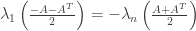and .

Second, applying the right half of the inequality gives

Matlab mod

if you would like to achieve something like this:

1 2 3 4->1 2 3 4

-1 0->2 4

5 6->1 2

you should use

mod(i-1,n)+1

where n=4

Graphical meaning of power of adjacency matrix

Set default initial page view in adobe reader

It’s not that easy, but I finally fixed it.

There are three options provided by Adobe Reader.

1. File->properties->Initial view
2. Edit->preferences->Page display->Default layout and zoom
3. Edit->preferences->Accessibility->Override page display

Many people recommend the second way, but it does not work for me.

The first option works, but only for one single PDF.

The third one works for all PDF for me!!! I found it here

http://superuser.com/questions/349971/how-do-i-set-default-view-preferences-in-adobe-acrobat

 

Summary: Useful Tikz commands

%% basics %%%%%%%%%%%%%%%%%%%%%%%%%%%%%%%%%%%%%%%%%%%%%%%%%%%%%%%%%
% define a variable
\def\length{3}

% coordinate
\coordinate (A)  at (0,0);
% relative coordinate: example
\draw ($(A)+(0,1)$) -- ($(A)+(1,0)$);

% arrow and text
\draw[->,thin] (A)--(A1) node[above] {$x$}; % the text x is beside the node A1
% arrow types
->
->>
-latex
-stealth
-angle 90 % looks like ->
% path and text 
\path (1) edge[bend left=7,->,sloped] node[near start]{\contour{white}{\tiny -1}  }(2);

Skew-symmetric in the complex case

Suppose S is a real skew-symmetric matrix; H is a real symmetric matrix.

For a real vector x, we have . But for a complex vector x, we do not have . Instead, we have

• is imaginary since (if the conjugate of a complex number has the opposite sign, then the complex number is imaginary)
• is real since (if the conjugate of a complex number is itself, then it is real)

 

 

 

 

Monotonicity of binomial coefficients

Here are two basic identities about the monotonicity of binormial coefficients

• for any
  In addition,
  For proof, see the post in stackexchange by Mario

• for any
  For proof, see the post in stackexchange

 

An example to illustrate mesh, surf

A Matlab example to illustrate mesh, surf, …

clc;clear;close all;
x_all=1:0.1:2;
y_all=5:0.5:10;
%
xNum=max(size(x_all));
yNum=max(size(y_all));
z_all=zeros(xNum,yNum);
for ix=1:xNum
    for iy=1:yNum
        x=x_all(ix);
        y=y_all(iy);
        z_all(ix,iy)=exp(x)*sin(y);
    end
end
%
[X,Y]=meshgrid(x_all,y_all); % don't care X or Y
surf(X,Y,z_all') % there is a transpose for z_all, otherwise the dimensions would not agree

Result:

 

Proof of the Henneberg construction and Laman graph

Memo:

The proof of the equivalence between Henneberg construction and the Laman graph:

http://www3.cs.stonybrook.edu/~jgao/CSE590-fall05/notes/lecture3.pdf

 

 

Matrix norm and spectral radius

Let be any norm of the nxn matrix A. Then

where is the spectral radius which is .

See reference or paper – The Rate of Convergence of a Matrix Power Series

Jordan Form – Generalized Eigenvector

Every matrix A can be written as

• We are already very familiar with the matrix , which can give us many useful insights.
• We are not very familiar with the matrix , which contains the generalized eigenvectors.

Every matrix has n linearly independent eigenvectors.

We use an example to demonstrate:

Then

Hence

1. 
2. 
3. 

Therefore,

1. is the normal eigenvector for . For each Jordan block, there is just one normal eigenvector. The normal eigenvector is always the first column of those corresponding to the Jordan block.
2. are the generalized eigenvectors. They can be computed by or . Note has two solutions: one is p_1 and the other is .

**********************************************************************************

In addition, note

Note is a special nilpotent matrix: shift matrix. We have

Therefore, the null space of is spanned by . So when computing , is the one that satisfies but . Since is zero, is just a vector that is linear independent to .

**********************************************************************************

The Jordan block is not necessarily as shown above. For example, it can have the form of

Then, every matrix is still similar to a modified Jordan matrix. The only difference is the norms of the generalized eigenvectors in are scaled by . For example, from

we have

and hence

Therefore, the previous generalized eigenvectors are still valid, we just need to scale them by . For example, suppose are the generalized eigenvectors for the case of , then for general we have the generalized eigenvectors as .

Note can be chosen differently for different Jordan block in a Jordan matrix. One option is to choose . See, for example, 1997- Two Results About the Matrix Exponential, Corollary 6

For example:

It has been verified by Matlab that

A useful inequality for eigenvalue and singular value

Let A be an arbitrary matrix. Suppose and .

General result:

For any k=1,…,n, we have

Special but very useful result:

Example:

Suppose A=S-I where S is skew-symetric. Note (A+A^T)/2=I.Then

Reference:

paper – 2000-singular values of matrix exponential, thm 1.4

 

Multiple solutions to a Lyapunov equation

Keywords: Lyapunov equation, unique solution, nonunique solution, stable matrix, Hurwitz matrix, controllability Gramian

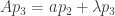
For the Lyapunov equation , it is well known that if A is stable, then the solution (controllability Gramian) is unique. Here I just give an example showing that if A is unstable, then it will have multiple solutions.

A =
 -1     1      1
 -1     0     0
 -1     0     0

B =
 1
 0
 0

W1 =
 0.5     0      0
 0       0.5    0
 0        0     0.5

W2 =
 0.5     0        0
 0      0.25    0.25
 0      0.25    0.25

It can be verified that

eig(A)=
 -0.5000 + 1.3229i
 -0.5000 - 1.3229i
 0.0000 + 0.0000i

So A has two negative eigenvalues and one zero eigenvalue.

• It can be verified that W1 and W2 both satisfy the Lyapunov equation!!
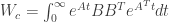
• In addition, W2 is the controllability Gramian by using the following code

tf=inf;
 fcnWc=@(x)expm(A*x)*B*B'*expm(A'*x);
 Wc=integral(fcnWc,0,tf,'ArrayValued',true)

Summarize the properties of AW+WA^T=-BB^T

For , three key conditions are:

(I) W>0
(II) A is stable
(III) (A,B) is controllable

To important conclusions:

• If W>0, then A is stable if and only if (A,B) is controllable! The proof is very simple based on the equation of shown below. See details here
• If A is stable, then W>0 if and only if (A,B) is controllable! That is because in this case W is the controllability Gramian. It is well known that W>0 if and only if (A,B) is controllable.

The first conclusion means that (I)+(II)->(III) and (I)+(III)->(II).
The second conclusion means that (II)+(I)->(III) and (II)+(III)->(I)

Therefore, the above two conclusions indicate that in the above three conditions, any two conditions imply the other condition. Hence the third conclusion, which may seem strange, is

• If (A,B) is controllable, then W>0 if and only if A is stable!

The third conclusion is simply equivalent to say (III)+(I)->(II) and (III)+(II)->(I), which have been proved to be correct by the first two conclusions.

Another way to summarize:

• (I)+(II)->(III): prove based on the equation of
• (I)+(III)->(II): prove based on the equation of or the controllability Gramian
• (II)+(III)->(I): prove based on the controllability Gramian

***********************************************************************************

Keywords: Lyapunov equation, negative stability, positive stability, Hurwitz

Problem: Given the Lyapunov equation

where W is positive definite and H is positive (semi-)definite. Now prove that A is positive (semi-)stable.

Conclusion: Suppose and . Note even for real matrix A, if its eigenvalue is complex, the eigenvector is also complex and we need to use conjugate transpose. One important conclusion is that

Clearly, if W is PD and H is PSD, then A is positive semi-stable. If W and H are both PD, then A is positive stable.

Detailed proof: See details here The proof is inspired by Topics in Matrix Analysis Lemma 2.4.5.

Structural controllability: How to Interpret Dilation and Cactus

Keywords: structural controllability, network controllability, stem, bud, cactus, dilation

How to Interpret Dilation and Cactus:

memo – structrual controllability

Matrix Exponential of Jordan Blocks

Here is a memo.

my memo

Key words: matrix exponential, Jordan block, Jordan canonical form

Singular values and diagonal entries of a PSD matrix

Fact:

Proof: note for all

Choose , then it can be seen that .

Similarly, we can show

For more complicated version, see Cauchy interlacing theorem.

Matrix condition number and angles between column vectors

keywords: matrix condition number, lower bound, angles between the column vectors, maximum and minimum singular values

memo

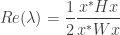
Which controllability Gramain is which Lyapunov equation’s solution??

For system x_dot=Ax+Bu, there are different definitions of the controllability Gramain and different definitions of the Lyapunov equations.

Fact:

is the soluton to

Proof:

Taking integral on both sides of the above equation gives

The left:

The right:

Therefore, the left and right give

QED

Remark: the above state is consistent with many papers and hence no need to worry about the correctness. In the past, I always thought the Gramian is the solution to the following one

But in fact it is not. The above Lyapunov equation can be obtained if you consider system x_dot=Ax and Lyapunov function V=x^TPx.

Real normal matrix

A complex matrix is normal if and only if or A can be unitarily diagonalizable , where * denotes the conjugate transpose or Hermitian transpose.

For a real matrix A, it is normal if and only if . In this case, how to prove it is equivalent to unitarily diagonalizable?

If , then

Note if there are complex matrices, use conjugate transpose instead of real transpose! In the above proof, if you use real transpose all the time, you cannot prove it.

*************************************************

By the way, any complex number can be mapped to a 2×2 matrix as

[a b;
-b a]

or

[a -b;
b a]

It is interesting that the 2×2 matrix is normal (it is a sum of an identity matrix and a skew-symmetric matrix, which are both normal and in the meantime commute). It can be shown that the sum and product of any two complex numbers can be equivalently expressed as the sum and product of two 2×2 matrices.